Understanding Latent Semantic Analysis

Introduction to LSA:#
LSA#
A classical problem in the field of natural language processing (NLP) is that of finding and matching semantic meaning from large bodies of text. Some classical solutions involve stemming, controlled vocabularies, and using thesauri 1. A different approach to this problem is Latent Semantic Analysis (LSA). LSA is an application of dimension reduction to the fields of natural language processing and information retrieval 2. Mathematically, it involves (1) creating a vector encoding of a large body of text, (2) computing a truncated singular value decomposition on the matrix, and (3) retrieving word and vector similarity in the dimension-reduced space. LSA is a well-studied model that remains an important tool and benchmark in the task of semantic similarity.
Mathematically, LSA finds a singular value decomposition for a term-document matrix. The term-document matrix can be constructed in varying ways based off of different document encoding methods. We can signify this matrix A(m*n) for m terms and n documents. The singular value decomposition of A is given by,A=U*sigma*V^T where sigma gives the sorted singular values of A and U and V are the decomposed sides of the term-document matrix. In a truncated SVD, we reduce the size of these matricies by taking only the k largest singular values and their respective vectors in U and V. As a result we find A_k, a rank k representation of our original term-document matrix.
Thus, the assumption of LSA is that semantically similar terms will be physically close together in the dimension-reduced space. Then, taking advantage of this distance, we can apply different algorithms to extract relationships between the documents. Moreover, the authors provide detailed argumentation as to why this type of dimension reduction parallels that used in the brain 3.
In this report, we look to describe, improve, and apply LSA. To begin, we provide a survey of the application of LSA to different NLP tasks and an experimental approach to understanding LSA in these settings. Next, we seek to improve and test different aspects of LSA and provide suggestions for some of the different variations available under the broader LSA framework. Finally, we attempt to prove the application of LSA in modern deep learning NLP models by inserting it as a re-weighting layer in the deepspeech pipeline.
Different LSA Tasks#
LSA, although frequently applied to the task of semantic indexing, can also be applied to other NLP tasks. By capturing the dimension-reduced space, we are better able to cluster and make predictions on the data. Some of these applications include: sentiment analysis, topic grouping, and document classification. LSA's ability to reduce the dimensionality of the data while retaining much of its latent meaning also makes it a useful tool in a diverse group NLP pipelines run on large datasets.
The application of LSA for sentiment analysis epitomizes its utility across a wide variety of NLP tasks. Generally, sentiment analysis refers to the task of extracting opinion or emotional data from text or image data. Modern semantic analysis models are often trained on huge labeled datasets of topic specific text. Recent models have become accurate enough to become useful models for guiding business decisions 4.
In this experiment, we will be using the Twitter US Airline Sentiment dataset accessed via Kaggle 5. As described by the original source, this dataset is,
A sentiment analysis job about the problems of each major U.S. airline. Twitter data was scraped from February of 2015 and contributors were asked to first classify positive, negative, and neutral tweets, followed by categorizing negative reasons (such as "late flight" or "rude service").
There exists some pre existing literature on the use of LSA for sentiment analysis. Wang and Wan 6 suggest a six part ML pipeline that involves cleaning the data, computing the SVD, deciding the polarity of the words, combining the word orientation, and finally running SVM classification on the resulting data. Using this method they were able to achieve reasonably accurate results.
To simplify the method, we will run the pipeline following:
- Clean data and find vector encodings.
- Find a dimension reduced SVD for all the data.
- Run kNN-Classification on the resulting dimension reduced SVD.
In running this pipeline with eight neighbors and reducing the term-document matrix to a rank 20 SVD, the algorithm achieved a classification accuracy of 70%. Obviously, this highly naive method for sentiment analysis failed to classify the tweets at a high rate. The sentiment breakdown of the original tweets was 63% negative, 16% positive, and 21% neutral. Therefore, the model did marginally better than had it always classified tweets as negative.
A similar task that utilizes LSA dimension reduced matrices is topic modeling. Topic modelling is an unsupervised learning method that is used to cluster documents based on their textual context. This definition is intentionally vague as topic modeling describes a class of algorithms and techniques applied to many different more specific NLP tasks. For example, the dimension-reduced clusters found using a topic modeling algorithm, when labels are provided, can be used to classify documents. The ability of these models to access latent information apparent in the documents makes them easy to apply to real-world problems. Po and Bergamaschi report a simple four stage method to extract movie recommendation data from plot summaries 7. The concept of topic modelling will be discussed in more detail in the Improving LSA section of this report.
Finally, among the most fundamental tasks solutions of which frequently utilize LSA is indexing and information retrieval. The final section of this report will focus on applying LSI (latent semantic indexing, synonymous to LSA) to improve pretrained STT models. The original LSI paper, Deerwester et. al 8, provides the following methods of document-document and term-term comparison. After having computed A_k=U_k*sigma_k*V^T_k, we find the term-to-term product matrix A*A^T=U_k*sigma^2_k*U^T_k and the document-to-document product matrix A^TA=V_k*sigma^2_k*V^T_k. The i,j value of this matrix represents the similarity score between the i*text{th} and j*text{th} term/document in the original term-document matrix. Finally, the authors provide a metric for creating a dimension-reduced representation of a document that doesn't exist in the original dataset. For original vector encoding of document p equal to X_p we can find a dimension reduced version under the constraint that transforming a vector in the matrix returns itself, V_p=X_p^T*U*sigma^-1
In these methods, LSA takes advantage of the distributional hypothesis which, in the context of linguistics, states that the semantic meaning of words in text can be understood by observing the context the words are found in 9. In applying this hypothesis, we are able to generate a thesaurus (in the form of the term-to-term product matrix) from only the latent features of documents.
Improving LSA:#
In this section, we examine and experiment on small adaptations to the LSA framework. All experiments will be performed on the topic classification/ modeling task, using the 20 newsgroup dataset 10. To reduce the datasets size for ease, we selected 5 of the 20 topics: atheism, graphics, car reviews, baseball, and space. These experiments will also replace traditional SVD with SKLearn's Randomized SVD (through 6 iterations) which is an implementation of Halko et. al 2009 11.
To begin, we performed a traditional LSA on the dataset. The kNN classifier (k=5) run on a rank 100 truncated SVD had an accuracy of 64%. We will use this number as our benchmark for future tests.
# 20 graphics terms with largest weight['edu', 'lines', 'subject', 'graphics', 'organization', 'image', 'com', 'university',\ 'jpeg', 'posting', 'host', 'file', 'nntp', 'software', 'data', 'use', \ 'writes', 'images', 'files', 'know']Across the experiments we find that the document encoding, ceteris paribus, had marginal affect on the model's accuracy. The classifier used however, made a major difference; Naive Bayes and SVM appeared as two viable options. In the final section, we find that all other attempted methods of dimension reduction fail to be computationally feasible for the large matrices required.
Document Encodings#
In the paper that introduced LSA as an NLP technique, the textual documents were encoded as count vectors. Additionally, the authors suggested performing a logarithmic transformation to regularize the vectors. However, it remains unclear whether the aforementioned encoding and transformation are appropriate in optimizing the model. In the next section, we lay out a framework and experimental results from routine experiments across different. Across all experiments we plan to use the same five topic subsample of the 20 news dataset reduced to 100 dimensions via SVD.
We compare two new vector encoding techniques: one-hot or binary encoding and TF-IDF. Likewise we compare different potential tranformations that can be applied to the standard word-count encoding. In each case, we ran the LSA model on the new term-document matrix and calculated the model's accuracy. Count and TF-IDF emerged as the two best encodings but only one-hot and the exponentially transformed vectors showed significantly different performance. A summary of the results is plotted below.
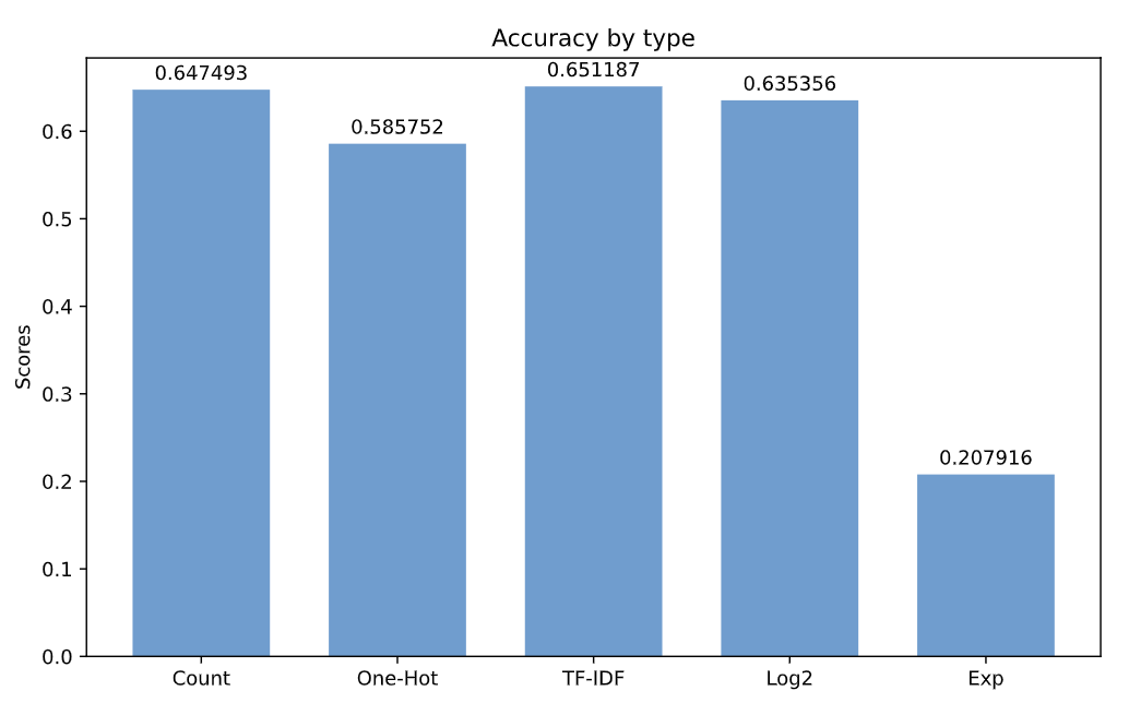
Overall, it appears that either TD-IFD or a transformed count vector serve as the highest performance encodings. That said, this experiment was only across one NLP task, one dataset, and didn't include other, more modern vector encodings.
Classifiers#
The final step in the topic classification task involves applying a classification algorithm on the dimension reduced representation of the textual data. In other areas of this report, kNN was used as the constant classification algorithm. However, kNN is a relatively naive classification algorithm and our results could potentially be improved by replacing the kNN classifier with other classes of algorithms. Under the same setting as the other experiments in this section, we test and compare the performance of the kNN classifier to that of multlinomial naive Bayes and linear SVM.
Although kNN provided an above-random classification performance, it was easily surpassed by the accuracy and generalization performance of the naive Bayes and linear SVM classifiers. Both of the newly introduced models achieved sub 10% error values on the test data. This result is visualized in the barr graph below.
![clf][(/img/blog/clf.png)]
Although this was a survey of just a small group of classifiers, our results show the importance of classifier selection. Moreover, it exemplifies the power of the LSA model; by reducing dimensionality of the model, we are able to linearly separate the topics into their respective groups and do so with a hight level of accuracy.
Ideal Dimensions#
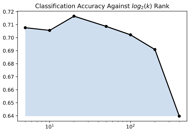
Another common problem when applying LSA is that of specifying the ideal number of dimensions of the transformed encoding. Being able to reduce the number of dimensions of the data, the word vectors in which could be tens of thousands of integers long, is the fundamental goal and property of the truncated SVD. However, removing too many dimensions could result in a representation that doesn't manage to accurately describe the dataset. The ideal number of output dimensions is a product of the input data, vector length, and sample size. In this section, we hope to provide a simple quick method to optimize the final output truncation.
The figure below, accessed from An Introduction to LSA, shows this phenomenon visually 3. In this experiment, they used LSA to find synonyms on a TOEFL dataset. They found that they maximized correctness when the data was reduced to ~300 dimensions.
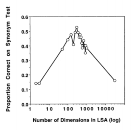
However, 300 is not a universal number, nor is 100 (the value originally suggested by the authors). Instead, careful tuning is important to ensure that the number of dimensions is correct. Here we provide a simple method to find a locally optimal number of dimension drawing ideas from SGD. In this case, however, we are able to only calculate the SVD once and upon each update remove more vectors from the decomposition.
def best_dim(train_X, train_Y, threshold = .01):    # Decide the number of components:    n_components = 100    if train_X.shape[0] > 5000:        n_components = 1000
    # Run SVD on the training data    U, sigma, VT = randomized_svd(train_encoding,                                n_components=1000,                                n_iter=6,                                random_state=None)
    # Train a kNN classifier on the truncated SVD    clf_knn = KNeighborsClassifier().fit(VT.T, train_Y) # Also customizable classifier, params    # Test data transformed    test_trans = test_encoding.T @ U @ np.diag(np.power(sigma, -1))    # Compute score    last = clf_knn.score(test_trans, test_Y)
    delta = -.1         # Arbitrary    increasing = False
    while delta > threshold:        n_components += (int) n_components \* delta
        # Train a kNN classifier on the truncated SVD        clf_knn = KNeighborsClassifier().fit(VT[:n_components].T, train_Y)        # Test data transformed        test_trans = test_encoding.T @ U[:n_components] @ np.diag(np.power(sigma[:n_components], -1))        # Compute score        temp = clf_knn.score(test_trans, test_Y)
return (last, n_components)Dimension Reduction#
In traditional LSA, the SVD is used to compute a lower dimension representation of the text encoding matrix. Under the general methodology of LSA, however, this step may be feasibly be replaced with other dimension reduction techniques. In this section, we attempted to replace the SVD with other methods of dimension reduction. Specifically, we ran a standard LSA pipeline simply replacing SVD with ISOMAP and metric MDS. All tests were run on the five topic subsample of the 20 news dataset.
Performing this experiment exposed one of the important reasons why the truncated SVD works well in this situation; It is one of the few dimension reduction methods that is computationally feasible for the huge matrices used in NLP. Other methods, like MDS and ISOMAP are computationally infeasible for matrices as small as the 70,000 * 3,000 term-document matrix used in this experiment. Moreover, SVD allows for a k-rank dimension reduction while other methods often perform best in n-to-2 or n-to-3 situations.
Applying LSA:#
I was not able to finish the code for this section, however, I find the idea interesting and hope to do more research into STT models in the future.
Concept#
The motivation of this section of this paper stems from the wide application of pretrained deep speech to text models (STT) in business applications. These models, although increasingly accurate, often struggle with generalization, make recurrent mistakes, and are difficult to tune to specific input data 12. For example, some models trained for normal speech recognition struggle when introduced to rare words. However, if a professor or orator is speaking in the topic-specific language of their field, the models often miss-simplify the person's speech resulting in decreased performance.
Most modern open source and commercial models have "boost" parameters or more advanced methods to allow businesses to fine tune models to their needs 13. These tools, however, often have to be pre-set and provide a one-time reweighting to the model. In many use cases however, an ideal model may dynamically adjust its weights during use as the topic of the speech changes. This type of reweighting requires a lightweight computationally simple solution.
LSA provides a simple method that could be used to dynamically adjust STT model weights as the topic of the speech changes.
Experiment#
To begin, we loaded the latest deepspeech library 14 into a docker environment with the standard pretrained English model. From empirical analysis, this model achieved 16% error on the Switchboard Hub5'00 dataset 15. Next, to get a benchmark on the model's unchanged state, we ran it on snippets of our dataset. The dataset in question is a collection of...
Conclusion#
LSA is a simple application of dimension reduction that serves as a key item in pipelines for a diverse group of NLP tasks. Despite being first documented over thirty years ago, it remains a powerful tool across many tasks.
References:#
- Dumais, S.T. (2004), Latent semantic analysis. Ann. Rev. Info. Sci. Tech., 38: 188-230. https://doi.org/10.1002/aris.1440380105↩
- Dumais, S. T., Furnas, G. W., Landauer, T. K., & Deerwester, S. (1988). Using latent semantic analysis to improve information retrieval. Proceedings of CHI'88 Conference on Human Factors in Computing Systems, 281–285.↩
- Landauer, T. K., Foltz, P. W., & Laham, D. http://lsa.colorado.edu/papers/dp1.LSAintro.pdf↩
- Usman Malik, https://stackabuse.com/python-for-nlp-sentiment-analysis-with-scikit-learn/↩
- Kaggle, https://www.kaggle.com/crowdflower/twitter-airline-sentiment↩
- Wang, Lan and Wan, Yuan. “Sentiment Classification of Documents Based on Latent Semantic Analysis.” Advanced Research on Computer Education, Simulation and Modeling, 2011, pp. 356–61.↩
- Bergamaschi, Sonia, and Po, Laura. “Comparing LDA and LSA Topic Models for Content-Based Movie Recommendation Systems.” Web Information Systems and Technologies, 2015, pp. 247–63.↩
- Deerwester, S., Dumais, S.T., Furnas, G.W., Landauer, T.K. and Harshman, R. (1990), Indexing by latent semantic analysis. J. Am. Soc. Inf. Sci., 41: 391-407. https://doi.org/10.1002/(SICI)1097-4571(199009)41:6<391::AID-ASI1>3.0.CO;2-9↩
- Firth, J.R. (1957). "A synopsis of linguistic theory 1930-1955". Studies in Linguistic Analysis: 1–32. Reprinted in F.R. Palmer, ed. (1968). Selected Papers of J.R. Firth 1952-1959. London: Longman.↩
- SK-Learn, https://scikit-learn.org/0.19/datasets/twenty_newsgroups.html↩
- Halko, et al., 2009 https://arxiv.org/abs/0909.4061↩
- Tits, Noé & El Haddad, Kevin & Dutoit, Thierry. (2020). Exploring Transfer Learning for Low Resource Emotional TTS. 10.1007/978-3-030-29516-5_5.↩
- Google Cloud STT documentation, https://cloud.google.com/speech-to-text/docs/adaptation-model↩
- Mozilla Deep Speech, https://github.com/mozilla/DeepSpeech↩
- Awni Hannun, Carl Case, Jared Casper, Bryan Catanzaro, Greg Diamos, Erich Elsen, Ryan Prenger, Sanjeev Satheesh, Shubho Sengupta, Adam Coates, & Andrew Y. Ng. (2014). Deep Speech: Scaling up end-to-end speech recognition. https://arxiv.org/abs/1412.5567.↩